Analyzing Data on Atmospheric Temperatures With R

About the data

I used the "temp_carbon," "greenhouse_gases," and "historic_co2" datasets from the dslabs library for this analysis. These three datasets contain data related to climate change over time. This data produces clear plots that demonstrate an increase in temperature, greenhouse gas levels, and carbon emissions from 800,000 years ago to modern times. All code is written in the R programming language. You can find the code here.

Modern temperature anomaly and carbon dioxide data: temp_carbon

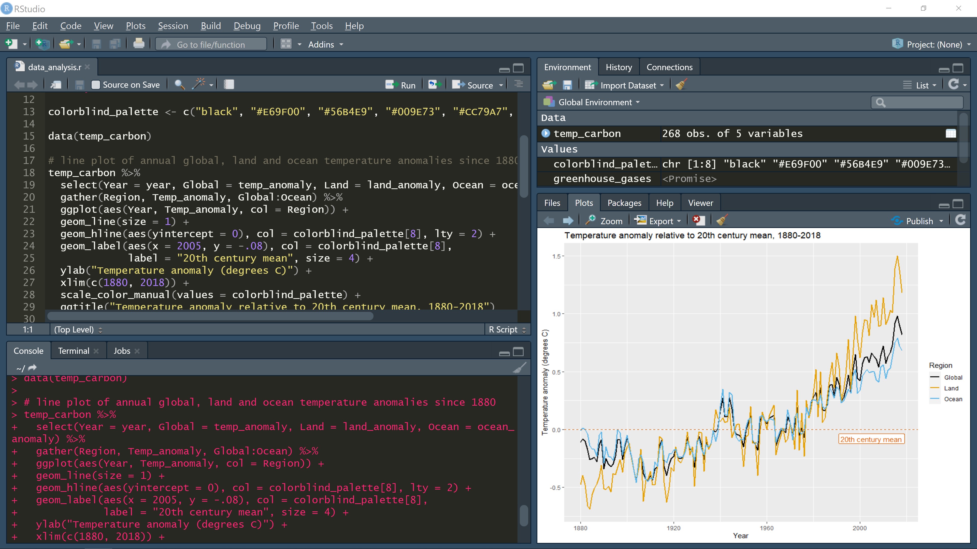
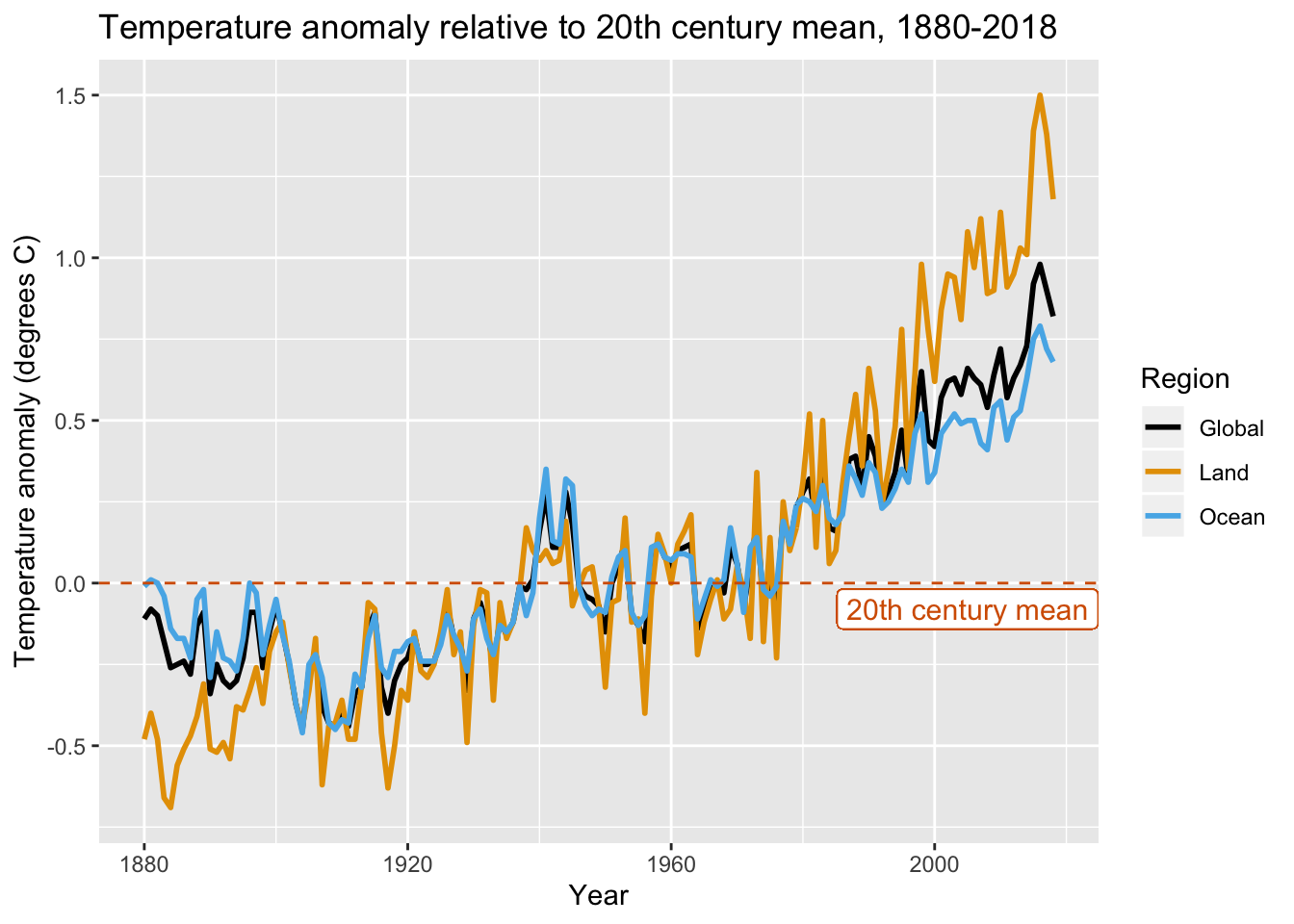
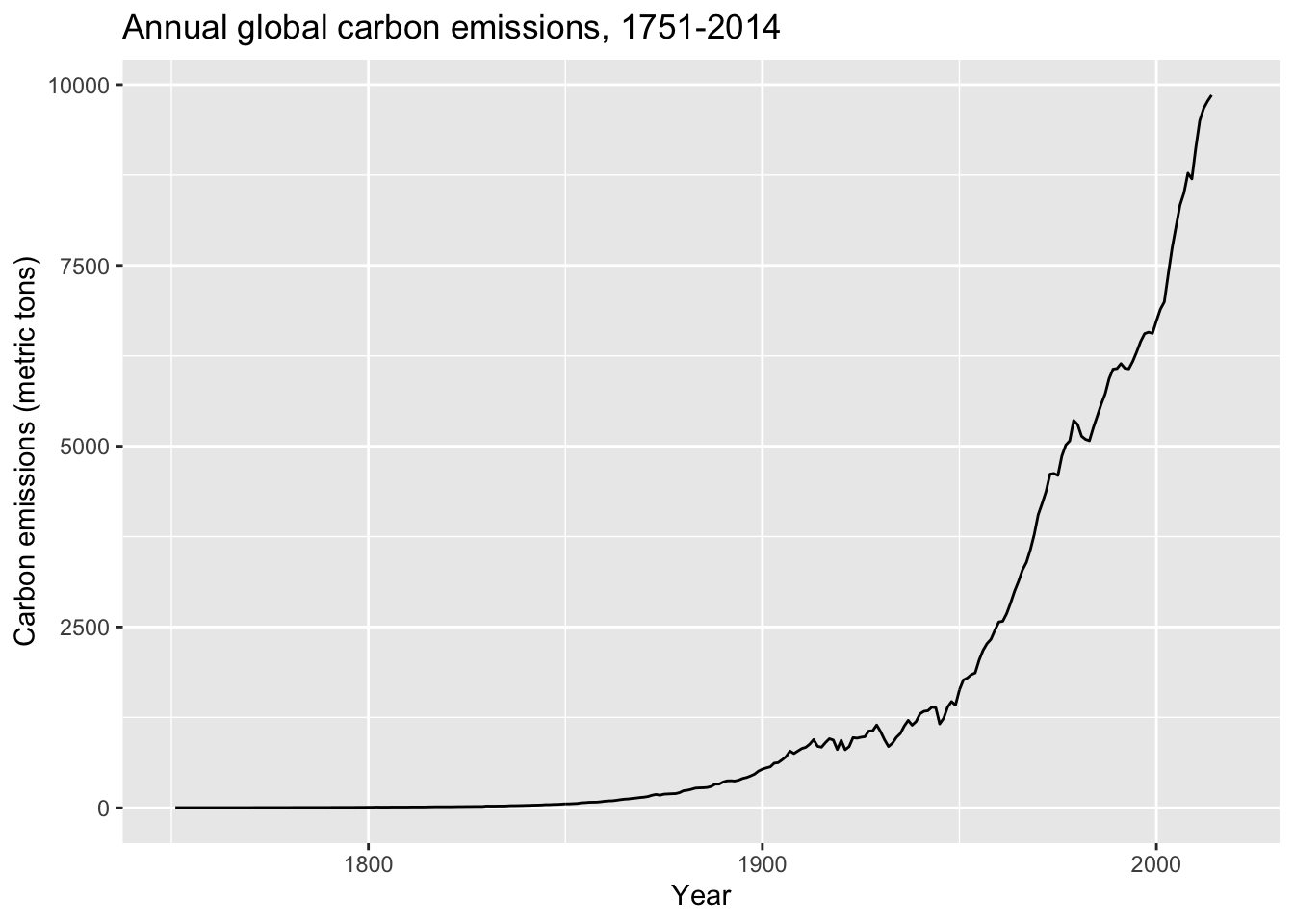
The temp_carbon dataset includes annual global temperature anomaly measurements in degrees Celsius relative to the 20th century mean temperature from 1880-2018. It includes anomalies over land and ocean. Additionally, it includes annual carbon emissions (in millions of metric tons) from 1751-2014. Temperature anomalies are from NOAA and carbon emissions are from Boden et al., via CDIAC.

data(temp_carbon)
                # line plot of annual global, land and ocean temperature anomalies since 1880
                temp_carbon %>%
                    select(Year = year, Global = temp_anomaly, Land = land_anomaly, Ocean = ocean_anomaly) %>%
                    gather(Region, Temp_anomaly, Global:Ocean) %>%
                    ggplot(aes(Year, Temp_anomaly, col = Region)) +
                    geom_line(size = 1) +
                    geom_hline(aes(yintercept = 0), col = colorblind_palette[8], lty = 2) +
                    geom_label(aes(x = 2005, y = -.08), col = colorblind_palette[8], 
                                label = "20th century mean", size = 4) +
                    ylab("Temperature anomaly (degrees C)") +
                    xlim(c(1880, 2018)) +
                    scale_color_manual(values = colorblind_palette) +
                    ggtitle("Temperature anomaly relative to 20th century mean, 1880-2018")

Greenhouse gas concentrations over 2000 years: greenhouse_gases

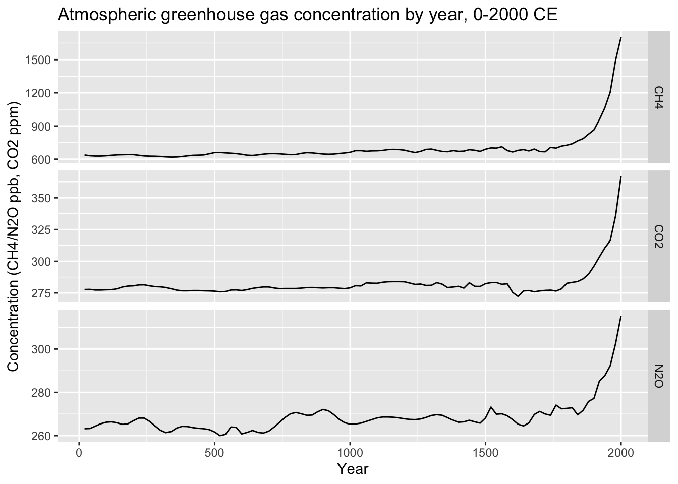
The greenhouse_gases data frame contains carbon dioxide (CO2, ppm), methane (CO2, ppb) and nitrous oxide (N2O, ppb) concentrations in 20 year invervals from 0-2000 CE. The data are a subset of ice core measurements from MacFarling Meure et al, via NOAA. We can see that there is a clear increase in all 3 gases starting around the time of the Industrial Revolution.

data(greenhouse_gases)
                # line plots of atmospheric concentrations of the three major greenhouse gases since 0 CE
                greenhouse_gases %>%
                    ggplot(aes(year, concentration)) +
                    geom_line() +
                    facet_grid(gas ~ ., scales = "free") +
                    xlab("Year") +
                    ylab("Concentration (CH4/N2O ppb, CO2 ppm)") +
                    ggtitle("Atmospheric greenhouse gas concentration by year, 0-2000 CE")

Compare this pattern with man made carbon emissions since the year 1751 from temp_carbon, which have risen in a similar way:

# line plot of anthropogenic carbon emissions over 250+ years
                temp_carbon %>%
                    ggplot(aes(year, carbon_emissions)) +
                    geom_line() +
                    xlab("Year") +
                    ylab("Carbon emissions (metric tons)") +
                    ggtitle("Annual global carbon emissions, 1751-2014")

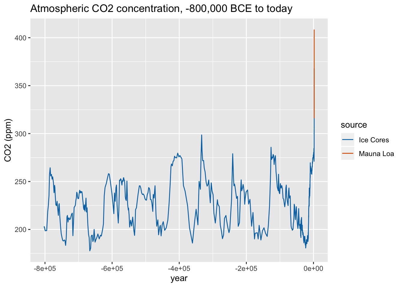
Carbon dioxide levels over the last 800,000 years: historic_co2

A common argument against the existence of anthropogenic climate change is that the Earth naturally undergoes cycles of warming and cooling governed by natural changes beyond human control. CO2 levels from ice cores and modern atmospheric measurements at the Mauna Loa observatory demonstrate that the speed and magnitude of natural variations in greenhouse gases pale in comparison to the rapid changes in modern industrial times. While the planet has been hotter and had higher CO2 levels in the distant past (data not shown), the current unprecedented rate of change leaves little time for planetary systems to adapt.

data(historic_co2)
                # line plot of atmospheric CO2 concentration over 800K years, colored by data source
                historic_co2 %>%
                    ggplot(aes(year, co2, col = source)) +
                    geom_line() +
                    ylab("CO2 (ppm)") +
                    scale_color_manual(values = colorblind_palette[7:8]) +
                    ggtitle("Atmospheric CO2 concentration, -800,000 BCE to today")